Quickstart#
An interactive session with IOSACal in Jupyter Notebook is the best way to get familiar with the software and create beautiful reports that are also self-explaining. Reproducible science!1
This is the standard import needed to start working with IOSACal and Jupyter Notebook:
from iosacal import R, combine, iplot
%matplotlib inline
Radiocarbon data#
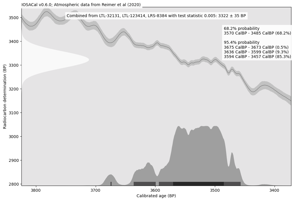
Now define three radiocarbon determinations and combine them:
rs = [R(3320, 65, 'LTL-32131'), R(3320,65,'LTL-123414'), R(3325,55,'LRS-8384')]
cr = combine(rs)
print(cr)
RadiocarbonSample( Combined from LTL-32131, LTL-123414, LRS-8384 with test statistic 0.005 : 3322 ± 35 )
Now that we have a combined age, calibrate it using the IntCal20 curve:
calcr = cr.calibrate('intcal20')
The calibrated date can be plotted as normal:
iplot(calcr)
Multiple dates#
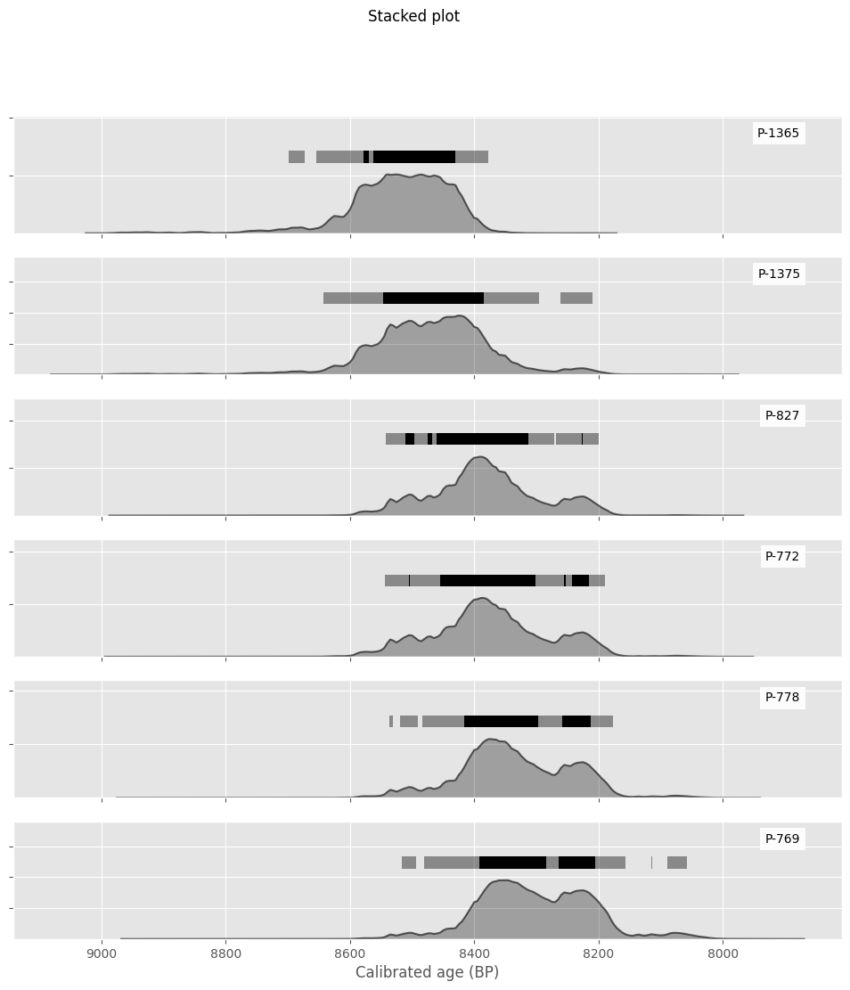
IOSACal can plot multiple dates for comparing, and you can use Python as normal
rs = [R(7729, 80, "P-1365"),
      R(7661, 99, "P-1375"),
      R(7579, 86, "P-827"),
      R(7572, 92, "P-772"),
      R(7538, 89, "P-778"),
      R(7505, 93, "P-769")]
multiple = [r.calibrate('intcal13') for r in rs]
It’s also possible to change Matplotlib settings without need to edit the underlying source code:
import matplotlib.pyplot as plt
plt.style.use('ggplot')
And create the resulting plot:
iplot(multiple)
Any plot can be saved directly to a file on disk, if needed:
iplot(multiple, output="Catalhöyük East level VI A.pdf")
This was a quick tour of IOSACal used interactively in Jupyter. Thank you!
- 1
This notebook can be downloaded as
quickstart.ipynb.